Britannia Beach
Tuesday, November 17 and Wednesday, December 2
Britannia Beach Community Hall, 101 Church Street
Howe Sound & Squamish
Explore flare and venting scenarios, change wind conditions, and compare concentrations across the study area.
2026 proposed application inputs and historical comparisons. Illustrative scenarios with assumed weather; not forecasts.
Preparing the map, controls and research data.
Meet the Woodfibre team to discuss the air-emissions and stormwater permits it has applied for. All four sessions run from 4:30–7:30 p.m. Pacific in 2026.
Tuesday, November 17 and Wednesday, December 2
Britannia Beach Community Hall, 101 Church Street
Thursday, November 19 and Thursday, December 3
Executive Suites, 40900 Tantalus Road
Official open-house notice from Woodfibre LNG ↗
Open the printable question sheet
The application now gives flare geometry. Will you confirm that it matches the installed equipment and publish the governing tip design, capacity, gas composition and exit conditions, together with the accepted Flaring Management Report and its engineering attachments?
2026 DMP · Table 6.2, p. 21Facility permit · conditions 14, 21–23
The application models up to 38 days of commissioning flaring. Over how many calendar months could that happen? How many hours of flaring and what volume of gas do you expect in each stage, including if startup has to be repeated?
2026 DMP · commissioning, Table 6.32026 notice · upset duration, p. 3
How do the proposed continuous HP/LP source rates fit the phrase “no routine flaring”? Which enforceable document defines the term here, and how are pilots, purge gas, passing valves, compressor seals and loading counted?
2026 notice · continuous sources, p. 2Facility permit · condition 14
The notice lists process upset and restart events of up to 24 hours and venting after a thermal oxidizer trip of up to 48 hours. How often do you expect each event? What happens if power is lost or the equipment takes longer to restart?
2026 notice · flaring and venting, p. 32026 DMP · durations, Table 6.5
The notice reports fine particles and total volatile organic compounds (VOCs). How much soot and benzene do you expect during a flare? During unburned venting, how much benzene and hydrogen sulphide could reach each community? Which pollutants have ambient objectives, permit limits or reporting requirements?
2026 notice · pollutant rates, pp. 2–3B.C. air quality objectives
What ground-level concentrations did your model predict for Britannia Beach, the estuary and each Squamish neighbourhood? Can you share the results by location and averaging period, with the wind direction, inversion conditions and background pollution for the highest values?
2026 application · air-quality assessment and modellingB.C. dispersion-modelling guideline
Will you show total concentrations from Woodfibre, the FortisBC compressor station, vessels and other relevant local sources, with existing air pollution included? Which overlapping startup, upset and shipping cases were assessed, and why?
2026 assessment · cumulative resultsBCER · FortisBC application notice
What continuous monitors will operate in town and along the transport corridor before, during and after startup? Who owns and quality-checks the data, how soon will it be public, and will an independent party have access to the raw records?
Woodfibre · regulatory filings and monitoring reportsB.C. air-quality data archive catalogue
Who checks an exceedance, who receives it and how quickly? What triggers investigation, operating changes and public advice? Will original readings, corrected data, permit contraventions and corrective actions remain publicly accessible?
Will you publish the accepted Flaring Notification Plan and show exactly how residents receive planned-event notices, unexpected-event updates and any health advice? Who is responsible, including outside business hours?
Compare communities and source cases ↓
Current and historical source cases
Compare the same assumed weather at ten reference points. Each column is a separate source contribution, without background pollution. These are air-layer averages, not forecasts of exposure at a home.
PM₂.₅ · 24-hour mean · µg/m³. Wind from 200° at 3 m/s; inversion cap 500 m above sea level.
The selected upset case holds its proposed maximum/design rate for 24 hours. It describes a process upset and restart, not commissioning. Historical rates, durations and source geometry differ.
On smaller screens, scroll the table sideways to compare all four cases.
| Community reference point | 2026 proposedHP flare · process upset / restart24 h release | Compressor maintenance2014 · 30 min | Tank shutdown2014 · 14 h | Feed-gas release2014 · 30 min |
|---|---|---|---|---|
| Squamish | 0.113 | 0.022 | 0.13 | <0.01 |
| Brackendale | 0.719 | 0.29 | 1.72 | <0.01 |
| Britannia Beach | <0.01 | <0.01 | <0.01 | <0.01 |
| Garibaldi Highlands | 0.19 | 0.0778 | 0.461 | <0.01 |
| Valleycliffe | 0.0442 | 0.0105 | 0.0625 | <0.01 |
| Dentville | 0.233 | 0.0624 | 0.37 | <0.01 |
| Garibaldi Estates | 0.298 | 0.0984 | 0.583 | <0.01 |
| The Northyards | 0.643 | 0.237 | 1.4 | <0.01 |
| Eagle Run | 0.611 | 0.235 | 1.4 | <0.01 |
| Northridge | 0.0794 | 0.0175 | 0.103 | <0.01 |
— Not reported for that source; not modelled. <0.01 Below the display precision in this selected scenario; not a zero-emission or no-exposure claim.
These saved calculations use the Explorer’s same transport engine and grid, with fixed winds for 24 hours, matching upper-level wind direction and particle removal switched off. Changing the selectors reads saved results; it does not change the simulator above.
The 2026 cases use current proposed rates and physical tip locations at 142.5 m above sea level. Historical cases use the earlier site proxy and 200 m injection height above model terrain. Changing source case therefore changes emissions, timing and geometry together. Flare plume rise, vent momentum, chemistry and background pollution are not calculated.
Each point samples its lowest model air layer, roughly 9–47 m deep at these reference points. It is not the highest concentration throughout a neighbourhood. The five wind settings do not represent every direction, wind reversal or event probability. Benchmark attainment and health risk require additional information.
PM₂.₅ uses the full-day mean. Other pollutants use the largest of 24 one-hour means; different places can reach their maximum in different hours. The detailed report retains the numerical checks and the full calculation records.
What changed in the 2026 source update? ↗ Proposed rates and physical tip locations now come from the application. The Explorer’s assumed winds are unchanged; flare buoyancy and vent momentum are not calculated.
Grid spacing affects plume width and peak concentration. Read the new transport accuracy check ↗
Elevation matters, but a plume does not simply follow the valley floor. Terrain channels air; a hot flare plume can rise into winds that differ from those below. An inversion can restrict vertical mixing. The direction of the wind at plume height matters as well as the wind felt at ground level.
Compare 24 hours and three wind settings across the study area. This dated CALMET calculation is separate from the illustrative Explorer above.
Compare separate heat-aware estimates for the three historical flare cases ↓
Possible health effects
Air pollution can worsen coughing, wheezing and breathing difficulties. Children, older adults and people with heart or lung conditions can be more affected. Health Canada: health effects · Who is more at risk.
Community comparison
A full-day PM₂.₅ average and a short peak answer different questions. The table uses a common time period for every place. Benchmark colours flag conditions to examine; they do not estimate the chance of illness.
Sources and methods
Review the proposed emission rates, source locations and durations behind each case. Read the current source audit ↗
The public tool is intended to compare conditional scenarios and explain potential exposure pathways. The map averages an air layer. Seven 2026 proposed source cases use application rates and physical tip geometry; the 2014 release reconstructions remain available separately. Winds are assumed, and the current-source calculation does not include flare buoyancy or vent momentum. A controlled test found substantial spreading caused by the calculation grid. Its footprint and peak concentrations change with resolution, so it cannot establish exposure at a home or a safe distance.
Time-varying releases, plume rise, representative local weather and background air remain priorities. The published application supplies more source information than the Explorer currently uses; a quantitative claim about likely local exposure also needs a suitable, tested transport calculation. The detailed evidence remains available below.
Reading the concentration colours
24-hour average; annual 98th percentile of daily averages. Annual objective: 8 µg/m³.
B.C. PM₂.₅ objectives ↗Annual 98th percentile of daily one-hour maxima, averaged over three years. Annual objective: 17 ppb.
B.C. NO₂ objectives ↗Annual 99th percentile of daily one-hour maxima, averaged over three years. Annual objective: 4 ppb.
B.C. SO₂ objectives ↗A single scenario cannot establish attainment or a permit breach. Compare total ambient concentration, including an appropriate background, over the matching period. Missing source or background data remain unknown. B.C. cautions that effects can occur below objectives. Provincial guidance
The 2026 combustion cases include SO₂. The vent case includes total VOC, H₂S and total reduced sulphur (TRS); TRS and H₂S must not be added as separate totals. Total VOC does not identify benzene, and NOx requires a stated conversion assumption for comparison with NO₂.
Flare comparison / Historical cases
Compare three historical designs using AERSCREEN, which accounts for flare heat and plume rise. These one-hour estimates are 1.5 m above flat ground, under assumed weather—not predictions for individual communities.
Loading comparison controls…
PM₂.₅ · largest sampled one-hour concentration (µg/m³)
Each value is the largest peak across 12 surface and temperature settings. The range below it shows how their peaks differ; it is not a confidence interval. Separate flare contributions, without background air pollution.
WWGF · 30 min historical release
Sampled peak range: 0.0847–0.165 µg/m³
LPCF · 14 h historical release
Sampled peak range: 6.9–22.2 µg/m³
CDGF · 30 min historical release
Provisional · flare-size warning
Sampled peak range: 9.4–23.3 µg/m³
Loading a case transfers its emissions and historical duration to the Explorer. The map uses assumed winds and release height; it does not use the heat-aware plume calculation shown in this comparison.
These are one-hour PM₂.₅ levels. B.C.’s 25 µg/m³ objective uses a 24-hour average, so these numbers cannot establish an exceedance or a pass.
The two 30-minute cases are held at their active release rate for a full hour here—twice their historical event mass. The tank case represents one active hour of its 14-hour release. These assumptions do not supply a town exposure forecast.
These are separate historical cases, not measured releases or current design rates. Changing a preset’s duration holds its rate fixed and changes total mass. NOx is expressed as NO₂ mass; total VOC does not identify individual compounds.
The historical engineering records also specify heat release. The browser map prescribes an injection height. Separate AERSCREEN calculations use the historical heat with synthetic weather and receptors 1.5 m above flat ground.
The concentration comparison multiplies each retained one-hour coefficient by that source’s reconstructed active pollutant rate, keeping its heat fixed. It does not change the map’s wind or release-height calculation. Valley flow, shoreline effects, chemistry and deposition are excluded. The compressor case’s equivalent diameter exceeds the model’s warning threshold; its result remains provisional.
The figure compares a passive pollutant released at 1 g/s while retaining each source’s full historical heat. Each distance selects its own maximum over assumed weather, so a curve does not describe one simultaneous plume. The compressor case retains an unresolved equivalent-diameter warning.
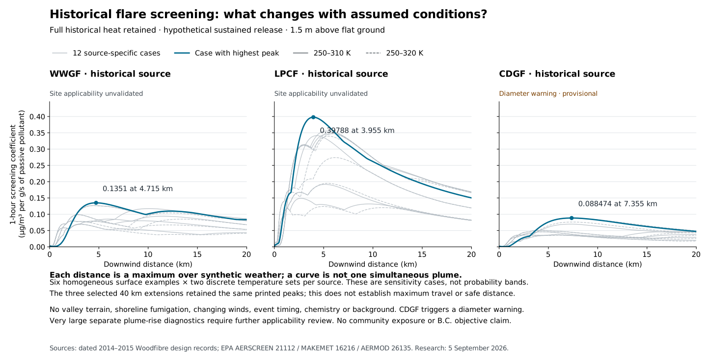
The coefficient is (µg/m³)/(g/s), not a community concentration. Changing pollutant mass at fixed heat is not a change in gas throughput; throughput changes also affect heat and plume rise.
Read the screening results and applicability limits ↗Research / Next steps
Prioritize information that could change the public assessment: release timelines, plume rise, local weather and background air. Keep further research separate from publishing a useful scenario tool.
The 2026 application supplies source rates, physical geometry and modelling parameters. Time-varying releases and a suitable plume-rise calculation are the next priorities.
Where to look Use the October 2026 source tables, reconcile the recorded heat-input discrepancy, and request event timelines and the accepted Flaring Management Report.
Close the gap when another analyst can reconstruct each release and its buoyancy or vent momentum.
Simultaneous source, shoreline and town weather, plus wind and temperature with height.
Where to look Obtain hourly source-site and town weather, plus documented inversion and outflow episodes. Prioritize evidence that changes the public scenario results.
Use inflow, outflow and weak-wind cases consistently across all communities; add observed episodes as their coverage is qualified.
Reviewed PM₂.₅, NO/NO₂/NOx, ozone and SO₂ with instrument details, clocks, missing values and event logs.
Where to look Build on the checked full-year onsite–town comparison by obtaining final hourly observations and dated instrument records.
Close the gap when the chosen background represents the intended receptors and matches the modelling period.
Individual VOCs, fuel sulfur, particle/soot fractions, and compatible FortisBC and vessel operating cases.
Where to look Request source calculations and testing methods; compare other projects only where fuel, flare design and conditions match.
Close the gap when pollutant conversion, background and concurrent sources have explicit evidence.
A suitable terrain and plume treatment, current ground elevations, public receptors and a complete run package.
Where to look Recover the original modelling files, evaluate local weather performance, then test source, numerical and chemistry sensitivity.
A flat-domain benchmark now quantifies numerical spreading. Resolve terrain sensitivity and plume-rise treatment before using the map for quantitative exposure estimates.
Occupied areas, Nation communities and sensitive public locations throughout the study area, with explicit concentration heights.
Where to look Cross-check public Nation, municipal and SLRD geography and facility directories; add points within small areas missed by the regular grid.
Apply the same pollutant, averaging-period, background and uncertainty criteria to every community.
Request drafts are unsent. No records request or hearing submission is sent by this website.
Research / Evidence
Our checks distinguish observed data, forecast output, historical engineering information and assumptions. The research notes include methods, failed checks and remaining gaps.
October 2026 rates, source geometry, durations and original documents. What changed in the Explorer, with historical inputs kept separate.
Transport benchmark · 29 SeptemberAn exact-solution test measures artificial plume spreading, compares finer grids and retains every failed check. Download the full experiment.
Review materials · 29 SeptemberModel distinctions, source provenance, runnable checks, unresolved results and focused review questions. AI-assisted verification; external scientific review pending.
Atmospheric profiles · 11 SeptemberSeparate temperature sampling and convective history, with whole-area comparisons and the earlier stability study.
Public weather data · 11 SeptemberArchived temperature, pressure and humidity recover detail lost in printed model files.
Wind calculation · 11 SeptemberCaptured calculation stages explain the large vertical-motion increment and the part cancelled by smoothing.
Explorer update · Historical inputsThe 14-hour tank-shutdown case joins two shorter releases, with explicit rates, event totals and averaging periods.
Model sensitivity · 11 SeptemberNine matched calculations retain the large vertical-motion excursion. Finer layers have not established more accurate local winds.
Independent model comparisonNative regional vertical winds provide a common reference across all nine configurations, with coverage and height limits retained.
Weather input methodsA source trace identifies the neutral fallback and the assumptions needed to test a different thermal treatment.
Model and observations · 11 SeptemberA common sampling method follows regional winds through the calculation and identifies where the airport mismatch is already present.
Engineering evidence · 2024 drawingA District-linked construction plan supplies a dated location candidate and specific leads for the current design records.
Model diagnosticConverting terrain-following winds under two explicit methods leaves large vertical excursions that still need physical evaluation.
Regional wind calculation · 11 SeptemberThree expanded-domain runs compare the whole study area, with maps and consistent results for every existing place reference.
Native weather inputsTwenty archive tiles resolve the model’s water categories and show which thermal fields are populated.
Exposure assessment designPublic reserve and land-use data reveal small areas missed by regular grid centres and guide the next receptor checks.
Observed · 2023–2025Six pollutants at Squamish Elementary, with daily timelines, missing-data checks and B.C. objective comparisons.
Research inputsCandidate concentrations by month and hour, checked ozone preparation, and the town monitor’s sampling context.
Observed · 2025Monthly PM₂.₅ and NO₂ comparisons across a year, with matching dates, measurement history and downloadable records.
Observed · 20258,730 paired hours provide a benchmark for testing the wind field.
Model and observations · June 2023A full month at the airport and Pam Rocks shows where modelled speed and direction differ from observations.
Model weather · 2023Regional weather profiles for Woodfibre and Squamish, with checks of the underlying grid and terrain.
Forecast tested against observationsSelected six-hour windows expose transport uncertainty, including a missed winter reversal.
Historical · Synthetic weatherDated flare inputs and a flat-ground calculation. No neighbourhood prediction follows.
Historical field comparisonTwo plume treatments compared with a year of stack observations: lower hourly error, but a larger average underestimate.
Modelling methodCurrent inputs, local validation, numerical checks, chemistry, background and independent review.
Methods, data & provenanceRead linked reports and download the supporting public research files.